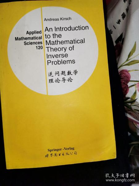
逆问题数学理论导论(英文版)
出版时间:
1999-10
版次:
1
ISBN:
9787506242516
定价:
42.00
装帧:
平装
开本:
其他
纸张:
胶版纸
页数:
282页
-
Following Keller [119] we call two problems inverse to each other if the formulation of each of them requires full or partial knowledge of the other. By this definition, it is obviously arbitrary which of the two problems we call the direct and which we call the inverse problem. But usually, one of the problems has been studied earlier and, perhaps, in more detail. This one is usually called the direct problem, whereas the other is the inverse problem. However, there is often another, more important difference between these two problems. Hadamard (see [91]) introduced the concept of a well-posed problem, originating from the philosophy that the mathematical model of a physical problem has to have the properties of uniqueness, existence, and stability of the solution. If one of the properties fails to hold, he called the problem iU-posed. It turns out that many interesting and important inverse problems in science lead to ill-posed problems,, while the corresponding direct problems are well-posed. Often, existence and uniqueness can be forced by enlarging or reducing the solution space (the space of "models"). For restoring stability, however, one has to change the topology of the spaces,which is in many cases impossible because of the presence of measurement errors. At first glance, it seems to be impossible to compute the solution of a problem numerically if the solution of the problem does not depend continuously on the data, i.e., for the case of ill-posed problems. Under additional a priori information about the solution, such as smoothness and bounds on the derivatives, however, it is possible to restore stability and construct efficient numerical algorithms. Preface
Introduction and Basic Concepts
1.1 Examples of Inverse Problems
1.2 I11-Posed Problems
1.3 The Worst-Case Error
1.4 Problems
2 Regularization Theory for Equations of the First Kind
2.1 A General Regularization Theory
2.2 Tikhonov Regularization
2.3 Landweber Iteration
2.4 A Numerical Example
2.5 The Discrepancy Principle of Morozov
2.6 Landweber‘s Iteration Method with Stopping Rule
2.7 The Conjugate Gradient Method
2.8 Problems
3 Regularization by Discretization
3.1 Projection Methods
3.2 Galerkin Methods
3.2.1 The Least Squares Method
3.2.2 The Dual Least Squares Method
3.2.3 The Bubnov-Galerkin Method for
Coercive Operators
3.3 Application to Symm's Integral Equation of the First Kind
3.4 Collocation Methods
3.4.1 Minimum Norm Colloction
3.4.2 Collocation of Symm's Equation
3.5 "Numerical Experiments for Symm's Equation
3.6 The Backus-Gilbert Method
3.7 Problems
4 Inverse Eigenvalue,Problems
4.1 Introduction
4.2 Construction of a Fundamental System
4.3 Asymptotics of the Eigenvalues and Eigenfunctions
4.4 Some Hyperbolic Problems
4.5 The Inverse Problem
4.6 A Parameter Identification Problem
4.7 Numerical Reconstrucion Techniques
4.8 Problems
5 An Inverse Scattering Problem
5.1 Introduction
5.2 The Direct Scattering problem
5.3 Properties of the Far Field Patterns
5.4 Uniqueness of the Inverse Problem
5.5 Numerical Methods
5.5.1 A Simplified Newton Method
5.5.2 A Modified Gradient Method
5.5.3 The Dual Space Method
5.6 Problems
A Basic Facts from Functional Analysis
A.1 Normed Spaces and Hilbert Spaces
A.2 Orthonormal Systems
A.3 Linear Bounded and Compact Operators
A.4 Sobolev Spaces of Periodi Functions
A.5 Spectral Theory for Compact Operators in Hilbert Spaces
A.6 The Frechet Derivative
B Proofs of the Results of Section 2.7
References
Index
-
内容简介:
Following Keller [119] we call two problems inverse to each other if the formulation of each of them requires full or partial knowledge of the other. By this definition, it is obviously arbitrary which of the two problems we call the direct and which we call the inverse problem. But usually, one of the problems has been studied earlier and, perhaps, in more detail. This one is usually called the direct problem, whereas the other is the inverse problem. However, there is often another, more important difference between these two problems. Hadamard (see [91]) introduced the concept of a well-posed problem, originating from the philosophy that the mathematical model of a physical problem has to have the properties of uniqueness, existence, and stability of the solution. If one of the properties fails to hold, he called the problem iU-posed. It turns out that many interesting and important inverse problems in science lead to ill-posed problems,, while the corresponding direct problems are well-posed. Often, existence and uniqueness can be forced by enlarging or reducing the solution space (the space of "models"). For restoring stability, however, one has to change the topology of the spaces,which is in many cases impossible because of the presence of measurement errors. At first glance, it seems to be impossible to compute the solution of a problem numerically if the solution of the problem does not depend continuously on the data, i.e., for the case of ill-posed problems. Under additional a priori information about the solution, such as smoothness and bounds on the derivatives, however, it is possible to restore stability and construct efficient numerical algorithms.
-
目录:
Preface
Introduction and Basic Concepts
1.1 Examples of Inverse Problems
1.2 I11-Posed Problems
1.3 The Worst-Case Error
1.4 Problems
2 Regularization Theory for Equations of the First Kind
2.1 A General Regularization Theory
2.2 Tikhonov Regularization
2.3 Landweber Iteration
2.4 A Numerical Example
2.5 The Discrepancy Principle of Morozov
2.6 Landweber‘s Iteration Method with Stopping Rule
2.7 The Conjugate Gradient Method
2.8 Problems
3 Regularization by Discretization
3.1 Projection Methods
3.2 Galerkin Methods
3.2.1 The Least Squares Method
3.2.2 The Dual Least Squares Method
3.2.3 The Bubnov-Galerkin Method for
Coercive Operators
3.3 Application to Symm's Integral Equation of the First Kind
3.4 Collocation Methods
3.4.1 Minimum Norm Colloction
3.4.2 Collocation of Symm's Equation
3.5 "Numerical Experiments for Symm's Equation
3.6 The Backus-Gilbert Method
3.7 Problems
4 Inverse Eigenvalue,Problems
4.1 Introduction
4.2 Construction of a Fundamental System
4.3 Asymptotics of the Eigenvalues and Eigenfunctions
4.4 Some Hyperbolic Problems
4.5 The Inverse Problem
4.6 A Parameter Identification Problem
4.7 Numerical Reconstrucion Techniques
4.8 Problems
5 An Inverse Scattering Problem
5.1 Introduction
5.2 The Direct Scattering problem
5.3 Properties of the Far Field Patterns
5.4 Uniqueness of the Inverse Problem
5.5 Numerical Methods
5.5.1 A Simplified Newton Method
5.5.2 A Modified Gradient Method
5.5.3 The Dual Space Method
5.6 Problems
A Basic Facts from Functional Analysis
A.1 Normed Spaces and Hilbert Spaces
A.2 Orthonormal Systems
A.3 Linear Bounded and Compact Operators
A.4 Sobolev Spaces of Periodi Functions
A.5 Spectral Theory for Compact Operators in Hilbert Spaces
A.6 The Frechet Derivative
B Proofs of the Results of Section 2.7
References
Index
查看详情
-
九五品
-
九五品
上海市虹口区
平均发货21小时
成功完成率100%
-
八五品
北京市海淀区
平均发货12小时
成功完成率98.05%
-
八品
北京市丰台区
平均发货16小时
成功完成率94.9%
-
九品
黑龙江省哈尔滨市
平均发货5小时
成功完成率93.04%
-
1999年 印刷
九品
上海市闵行区
平均发货15小时
成功完成率88.17%
-
八五品
广东省东莞市
平均发货7小时
成功完成率91.61%
-
九五品
北京市东城区
平均发货26小时
成功完成率85.12%
-
九品
山东省烟台市
平均发货4小时
成功完成率93.56%